Devils Hole

Introduction

This vignette demonstrates the usage of isogeochem using a case study based on Bajnai et al. (2021).

Background:

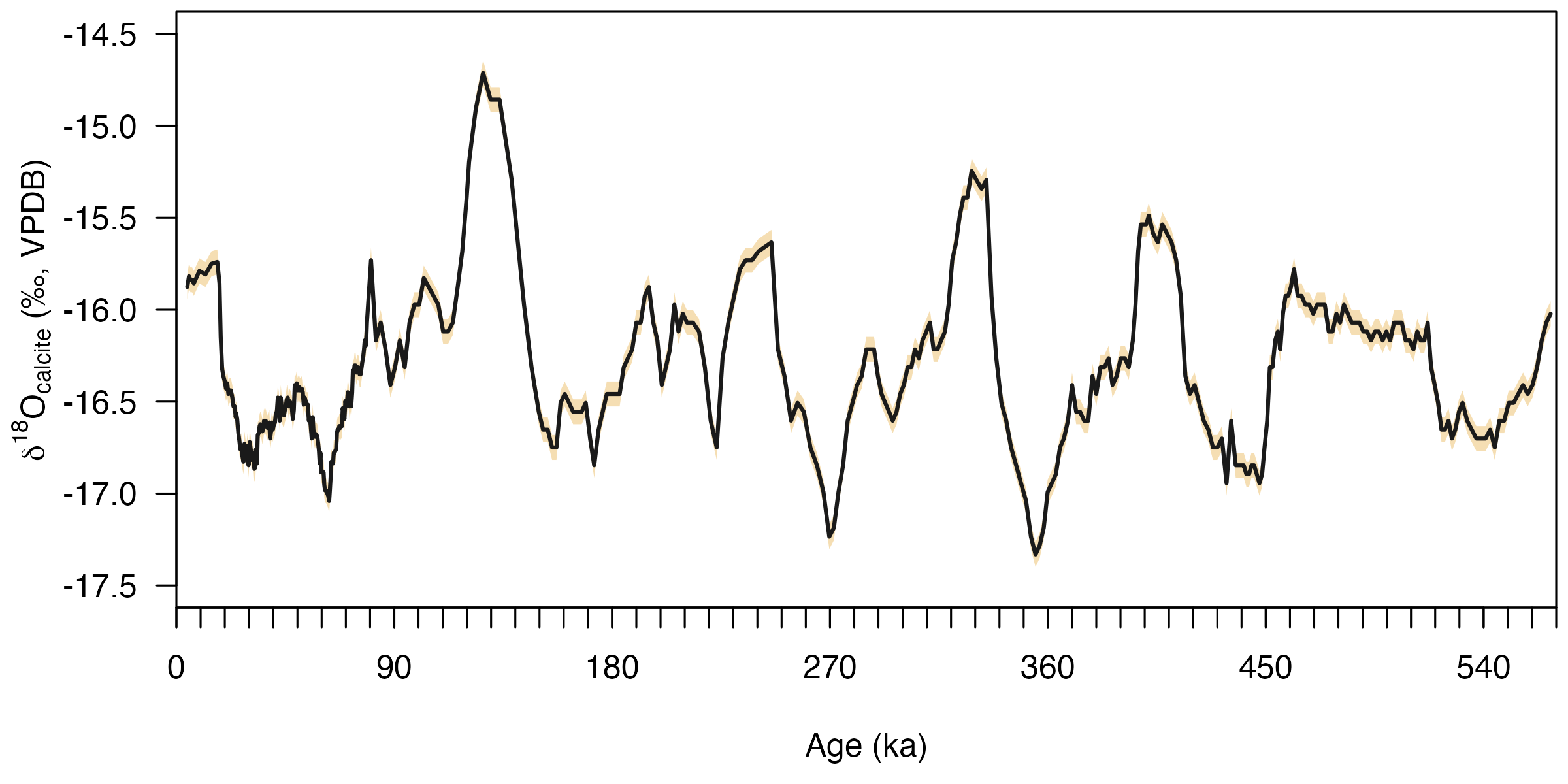
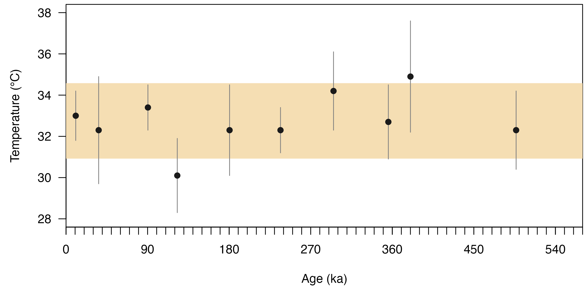
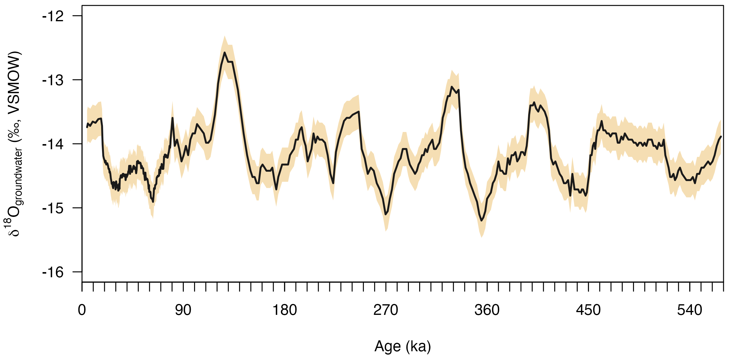
Winograd et al. (2006) acquired a δ¹⁸O time series from carbonates that precipitated underwater in the Devils Hole caves spanning the last ca. 570 thousand years. Now, we are interested in the variations in the δ¹⁸O value of the groundwater in this period. To reconstruct a groundwater δ¹⁸O time series from the carbonate δ¹⁸O values, we have to know the temperature of the groundwater. Therefore, we measured the clumped isotope values of ten calcite samples. First, we convert the measured ∆₄₇ values to carbonate growth temperatures. Then, using the mean of the clumped isotope temperatures, we convert the carbonate δ¹⁸O time series to a groundwater δ¹⁸O time series.

Package setup

Download, install, and load the isogeochem package:

if (!require("isogeochem")) install.packages("isogeochem")
library("isogeochem")

Load data

Data can be loaded into R in many ways. For example, to load data from an excel file you could use the openxlsx package. For this vignette, however, lets specify the measured ∆₄₇ values manually:

# D47(CDES90) values of Devils Hole carbonates 
DH_D47     = c(0.573, 0.575, 0.572, 0.581, 0.575, 0.575, 0.570, 0.574, 0.568, 0.575)
DH_D47_err = c(0.003, 0.007, 0.003, 0.005, 0.006, 0.003, 0.005, 0.005, 0.007, 0.005)
DH_D47_age = c(10.70, 36.00, 90.35, 122.75, 180.45, 236.65, 295.15, 355.65, 380.05, 496.65)

There are datasets available in isogeochem, which can be used simply by typing their name. For example, the devilshole dataset includes the original δ¹⁸O composite time series from the Devils Hole caves.

DH_age        = devilshole$age
DH_d18O_VSMOW = devilshole$d18O_VSMOW
DH_d18O_err   = devilshole$d18O_error

Carbonate δ¹⁸O vs age

Lets visualize the carbonate δ¹⁸O VPDB time series:

# Convert d18O VSMOW values to the VPDB scale 
DH_d18O_VPDB = to_VPDB(DH_d18O_VSMOW)

# Calculate the errors
DH_d18O_VPDB_err1 = to_VPDB(DH_d18O_VSMOW + DH_d18O_err)
DH_d18O_VPDB_err2 = to_VPDB(DH_d18O_VSMOW - DH_d18O_err)

# Plot the results
plot(0, type = "l" , las = 1, xaxs = "i", xaxt = "n", 
     ylim = c(-17.5, -14.5),
     xlim = c(0, 570), 
     ylab = expression(delta ^ 18 * "O"[calcite] * " (‰, VPDB)"),
     xlab = "Age (ka)")

# Set up the x axis with ticks and labels
axis(1, at = seq(0, 570, by = 90))
axis(1, at = seq(0, 570, by = 10), labels=NA)

# Add the error interval the plot
polygon(c(DH_age, rev(DH_age)), c(DH_d18O_VPDB_err1, rev(DH_d18O_VPDB_err2)),
        col="wheat", border = NA)

# Add the carbonate d18O VPDB time series to the plot
lines(DH_age, DH_d18O_VPDB, lwd=2, col="gray10")

Calculate growth temperatures from ∆₄₇

# Convert D47 values into temperatures using the equation in Fiebig et al. (2021)
DH_temp = temp_D47(DH_D47, DH_D47_err, eq = "Fiebig21")
DH_temp_mean = mean(DH_temp$temp)
DH_temp_mean
#> [1] 32.75
DH_temp_err  = mean(DH_temp$temp_err)
DH_temp_err
#> [1] 1.83

# Plot the results
plot(0, type = "l", las = 1, xaxt = "n", xaxs = "i",
     ylim = c(28, 38),
     xlim = c(0, 570),
     ylab = "Temperature (°C)",
     xlab = "Age (ka)")

# Set up the x axis with ticks and labels
axis(1, at = seq(0, 570, by = 90))
axis(1, at = seq(0, 570, by = 10), labels = NA)

# Add mean error range
rect(0, DH_temp_mean - DH_temp_err,
     570, DH_temp_mean + DH_temp_err,
     col = "wheat", border = NA)

# Add error bars
segments(DH_D47_age, DH_temp$temp - DH_temp$temp_err,
         DH_D47_age, DH_temp$temp + DH_temp$temp_err, col = "gray50")

# Add points
points(DH_D47_age, DH_temp$temp, col = "gray10", pch = 19)

Groundwater δ¹⁸O versus age

The calculated clumped isotope temperatures for the samples are statistically indistinguishable, which allows us to calculate a mean groundwater temperature and use that to reconstruct the variations in groundwater δ¹⁸O.

# Calculate groundwater d18O values and its error
DH_d18O_gw = d18O_H2O(
  temp = DH_temp_mean,
  d18O_c_VSMOW = DH_d18O_VSMOW,
  min = "calcite",
  eq = "Coplen07")
DH_d18O_gw_err_low = d18O_H2O(
  temp = DH_temp_mean + DH_temp_err,
  d18O_c_VSMOW = DH_d18O_VSMOW - DH_d18O_err,
  min = "calcite",
  eq = "Coplen07")
DH_d18O_gw_err_high = d18O_H2O(
  DH_temp_mean - DH_temp_err,
  DH_d18O_VSMOW + DH_d18O_err,
  min = "calcite",
  eq = "Coplen07")

# Plot the results
plot(0, type = "l", las = 1, xaxt = "n", xaxs = "i",
     ylim = c(-16, -12),
     xlim = c(0, 570),
     ylab = expression(delta ^ 18 * "O"[groundwater] * " (‰, VSMOW)"),
     xlab = "Age (ka)")

# Set up the x axis with ticks and labels
axis(1, at = seq(0, 570, by = 90))
axis(1, at = seq(0, 570, by = 10), labels = NA)

# Add the error interval the plot
polygon(c(DH_age, rev(DH_age)), c(DH_d18O_gw_err_low, rev(DH_d18O_gw_err_high)),
        col = "wheat", border = NA)

# Add the carbonate d18O time series to the plot
lines(DH_age, DH_d18O_gw, lwd = 2, col = "gray10")